Safely Deploying ML Models to Production: Four Controlled Strategies (A/B, Canary, Interleaved, Shadow Testing)

admin 3 hours ago

0 0 7 minutes read

Safely Deploying ML Models to Production: Four Controlled Strategies (A/B, Canary, Interleaved, Shadow Testing)

Deploying a new machine learning model to production is one of the most important phases of the ML lifecycle. Even if the model works well in validating and testing data sets, directly replacing an existing production model can be risky. Offline experiments rarely capture the full complexity of a real-world environment—data distributions can change, user behavior can change, and system constraints on productivity can differ from those in controlled trials.

As a result, a model that appears superior during development may degrade performance or negatively impact the user experience once deployed. To mitigate these risks, ML teams use controlled release techniques that allow them to test new models under real production conditions while minimizing potential disruptions.

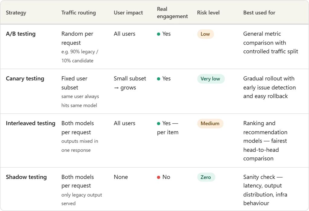
In this article, we examine four widely used techniques—A/B testing, Canary testing, mid-range testing, and Shadow testing—that help organizations safely deploy and validate new machine learning models in production environments.

A/B testing

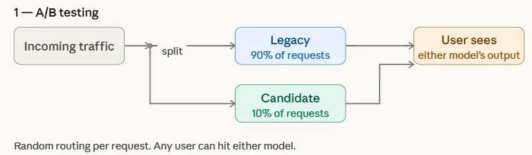
A/B testing is one of the most widely used methods for safely introducing a new machine learning model into production. In this way, incoming traffic is divided between two versions of the system: existing inheritance model (control) and candidate model (transformation). Often the distribution is uneven to limit risk—for example, 90% of applications may continue to be assigned to the legacy model, while only 10% are transferred to the candidate model.

By exposing both models to real-world traffic, teams can compare downstream performance metrics such as click-through rate, conversion, engagement, or revenue. This controlled test allows organizations to test whether a candidate model really improves results before gradually increasing its share of traffic or fully replacing a legacy model.

Canary test

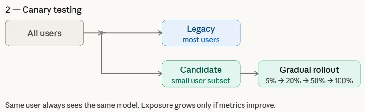
Canary test a controlled release strategy where a new model is first used for a small set of users before it is gradually rolled out to all users. The name comes from an old mining operation where miners carried canaries into coal mines to detect toxic gases—the birds were the first to react, warning the miners of danger. Similarly, in machine learning applications, i candidate model initially exposed to a limited group of users while the majority continue to be used by inheritance model.

Unlike A/B testing, which randomly allocates traffic to all users, canary testing targets a specific subset and gradually increases exposure if performance metrics show success. This gradual rollout helps teams spot problems early and roll back quickly if necessary, reducing the risk of widespread impact.

Inadequate Testing

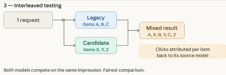
Intermediate assessment tests multiple models by mixing their results within the same feedback displayed to users. Instead of submitting every request to a legacy or candidate model, the system combines predictions from both models in real time. For example, in a recommendation system, some items on the recommendation list may appear in inheritance modelwhile others are made by candidate model.

The system then logs engagement signals—such as click-through rate, view time, or negative feedback—for each recommendation. Because both models are tested within the same user interface, cross-sectional testing allows groups to compare performance directly and efficiently while minimizing bias caused by differences in user groups or traffic distribution.

Shadow Test

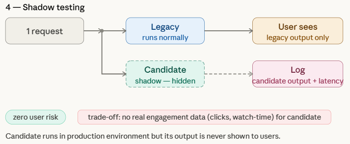
A shadow testalso known as shadow posting or dark initiationit allows teams to test a new machine learning model in a real production environment without affecting the user experience. In this method, the candidate model runs parallel to inheritance model and receives the same live requests as the production system. However, only legacy model predictions are returned to users, while candidate model outputs are logged for analysis.

This setup helps teams test how the new model behaves under real-world traffic and infrastructure conditions, which are often difficult to replicate in offline testing. Shadow testing provides a low-risk way to measure a candidate model against a legacy model, although it can’t capture true user interaction metrics—such as clicks, view time, or conversions—since your predictions can’t be displayed to users.

Simulation Techniques Using ML Modeling

We are preparing

Before simulating any strategy, we need two things: a way to represent the incoming requests, and a position in each model.

Each model is simply a function that takes a request and returns a score — a number that loosely represents how good that model’s recommendation is. The legacy model’s score is set at 0.35, while the candidate model reaches 0.55, which makes the candidate better on purpose to ensure that each strategy gets improved.

make_requests() generates 200 requests spread across 40 users, giving us enough traffic to see meaningful differences between techniques while keeping the simulation lightweight.

import random
import hashlib
 
random.seed(42)


def legacy_model(request):
    return {"model": "legacy",    "score": random.random() * 0.35}
 
def candidate_model(request):
    return {"model": "candidate", "score": random.random() * 0.55}
 
def make_requests(n=200):
    users = [f"user_{i}" for i in range(40)]
    return [{"id": f"req_{i}", "user": random.choice(users)} for i in range(n)]
 
requests = make_requests()

A/B testing

ab_route() is the core of this strategy — for every incoming request, it draws a random number of routes to the candidate model only if that number falls below 0.10, otherwise the request goes to legacy. This gives the candidate about 10% of the traffic.

We then collect the prediction scores for each model separately and calculate the average at the end. In a real system, these points will be replaced by real engagement metrics like click-through rate or watch time – here the points simply represent “how good this recommendation was.”

print("── 1. A/B Testing ──────────────────────────────────────────")
 
CANDIDATE_TRAFFIC = 0.10   # 10 % of requests go to candidate
 
def ab_route(request):
    return candidate_model if random.random() < CANDIDATE_TRAFFIC else legacy_model
 
results = {"legacy": [], "candidate": []}
for req in requests:
    model  = ab_route(req)
    pred   = model(req)
    results[pred["model"]].append(pred["score"])
 
for name, scores in results.items():
    print(f"  {name:12s} | requests: {len(scores):3d} | avg score: {sum(scores)/len(scores):.3f}")

Canary test

The main function here is get_canary_users(), which uses an MD5 hash to assign users to the canary group. The key word is deterministic – sorting users by their hash means that the same users are always in the canary group in every run, which shows how a real canary deployment works when a specific user always sees the same model.

We then simulated three phases by simply increasing the proportion of canary users — 5%, 20%, and 50%. For each request, the route is determined by whether the user belongs to the canary group, not by a random coin flip as in A/B testing. This is the basic difference between the two techniques: A/B testing is split by request, canary testing is split by user.

print("n── 2. Canary Testing ───────────────────────────────────────")
 
def get_canary_users(all_users, fraction):
    """Deterministic user assignment via hash -- stable across restarts."""
    n = max(1, int(len(all_users) * fraction))
    ranked = sorted(all_users, key=lambda u: hashlib.md5(u.encode()).hexdigest())
    return set(ranked[:n])
 
all_users = list(set(r["user"] for r in requests))
 
for phase, fraction in [("Phase 1 (5%)", 0.05), ("Phase 2 (20%)", 0.20), ("Phase 3 (50%)", 0.50)]:
    canary_users = get_canary_users(all_users, fraction)
    scores = {"legacy": [], "candidate": []}
    for req in requests:
        model = candidate_model if req["user"] in canary_users else legacy_model
        pred  = model(req)
        scores[pred["model"]].append(pred["score"])
    print(f"  {phase} | canary users: {len(canary_users):2d} "
          f"| legacy avg: {sum(scores['legacy'])/max(1,len(scores['legacy'])):.3f} "
          f"| candidate avg: {sum(scores['candidate'])/max(1,len(scores['candidate'])):.3f}")

Inadequate Testing

Both models apply to the entire request, and interleave() interleaves their output by alternating objects — one from legacy, one from candidate, one from legacy, and so on. Each item is tagged with its source model, so when a user clicks on something, we know exactly which model to pay for.

A small amount of random noise (-0.05, 0.05) added to each item’s output mimics the natural variation you would see in real samples — two items from the same model will not have the same quality.

Finally, we calculate the CTR separately for each model item. Because both models are competing for the same requests against the same users at the same time, there is no confounding factor — any difference in CTR is down to the quality of the model. This is what makes the mean test a statistically pure comparison of four strategies.

print("n── 3. Interleaved Testing ──────────────────────────────────")
 
def interleave(pred_a, pred_b):
    """Alternate items: A, B, A, B ... tagged with their source model."""
    items_a = [("legacy",    pred_a["score"] + random.uniform(-0.05, 0.05)) for _ in range(3)]
    items_b = [("candidate", pred_b["score"] + random.uniform(-0.05, 0.05)) for _ in range(3)]
    merged  = []
    for a, b in zip(items_a, items_b):
        merged += [a, b]
    return merged
 
clicks = {"legacy": 0, "candidate": 0}
shown  = {"legacy": 0, "candidate": 0}
 
for req in requests:
    pred_l = legacy_model(req)
    pred_c = candidate_model(req)
    for source, score in interleave(pred_l, pred_c):
        shown[source]  += 1
        clicks[source] += int(random.random() < score)   # click ~ score
 
for name in ["legacy", "candidate"]:
    print(f"  {name:12s} | impressions: {shown[name]:4d} "
          f"| clicks: {clicks[name]:3d} "
          f"| CTR: {clicks[name]/shown[name]:.3f}")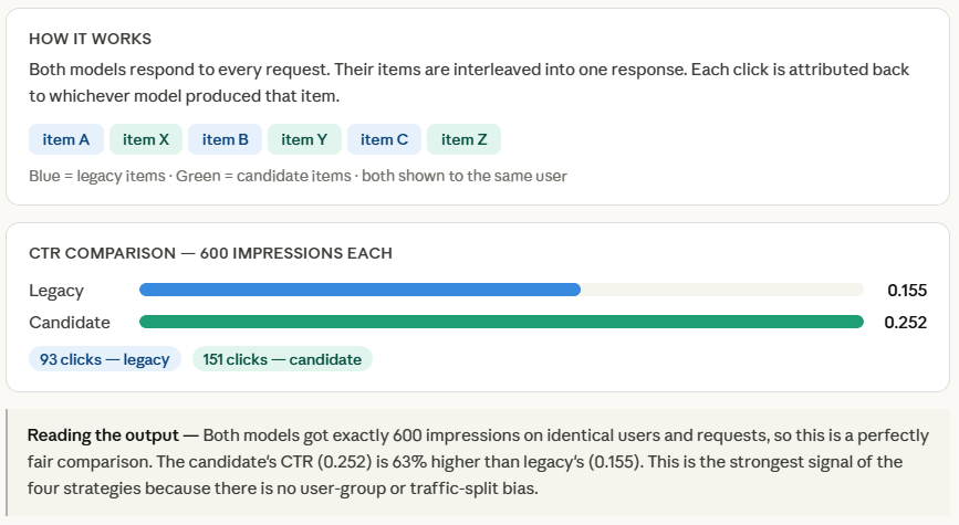

Shadow Test

Both models work for the entire application, but the loop makes a clear difference – live_pred is what the user gets, shadow_pred goes directly to the log and nothing else. Candidate output is not returned, displayed, or processed. The log list is the whole point of shadow testing. In a real system this will be written to a database or data warehouse, and developers will later query it to compare long-term distributions, output patterns, or point distributions against a legacy model – all without affecting a single user.

print("n── 4. Shadow Testing ───────────────────────────────────────")
 
log = []   # candidate's shadow log
 
for req in requests:
    # What the user sees
    live_pred   = legacy_model(req)
 
    # Shadow run -- never shown to user
    shadow_pred = candidate_model(req)
 
    log.append({
        "request_id":       req["id"],
        "legacy_score":     live_pred["score"],
        "candidate_score":  shadow_pred["score"],    # logged, not served
    })
 
avg_legacy    = sum(r["legacy_score"]    for r in log) / len(log)
avg_candidate = sum(r["candidate_score"] for r in log) / len(log)
 
print(f"  Legacy    avg score (served):  {avg_legacy:.3f}")
print(f"  Candidate avg score (logged):  {avg_candidate:.3f}")
print(f"  Note: candidate score has no click validation -- shadow only.")

Check out Full Notebook Here. Also, feel free to follow us Twitter and don’t forget to join our 120k+ ML SubReddit and Subscribe to Our newspaper. Wait! are you on telegram? now you can join us on telegram too.

I am a Civil Engineering Graduate (2022) from Jamia Millia Islamia, New Delhi, and I am very interested in Data Science, especially Neural Networks and its application in various fields.

admin 3 hours ago

0 0 7 minutes read